Credit Scoring Series Part Three: Data Preparation and Exploratory Data Analysis
In computer science, there’s an axiom that rings especially true when it comes to data projects: “Garbage in, garbage out.” In every case – and especially in credit scorecard development – data preparation is paramount. And unfortunately, data preparation is the most challenging, time-consuming phase of the Cross Industry Standard Process for Data Mining (CRISP-DM) cycle. In most projects, teams dedicate 70% of their time to data preparation; in some cases, that figure can reach more than 90%. That’s because data preparation involves data collection, combining multiple data sources, aggregations, and transformations, data cleansing, “slicing and dicing,” and looking at the data’s breadth and depth so organizations can clearly understand how to turn data quantity into data quality. Ensuring quality data preparation helps teams move to the next phase of scorecard development – model building.
This series’ previous article discussed the importance of model design and identified its main components: unit of analysis, population frame, sample size, criterion variable, modeling windows, data sources, and data collection methods. It’s vital to consider each of these components for successful data preparation. The final product of this stage is a mining view that encompasses the right level of analysis, modeling population, and independent and dependent variables.
| Mining view component | Application scorecard case study example |
|---|---|
| Unit of analysis | Customer level |
| Population frame | Loan applicants with previous bad debt history |
| Sample size | Through the door applicants during 2015 and 2016 |
| Data sources | Credit bureau data, applicant data, age debt history |
| Independent variables | Mixture of nominal, ordinal and interval data, such as aggregated values, flags, ratios, time and date values |
| Dependent variable | Default status (1 or 0) |
| Operational definitions | Default: 90 days past due |
| Observation window | Historical credit bureau customer information over the period of three years |
| Performance window | One year |
Table 1. Model design components
Data Sources
As the old saying goes, the more the merrier. As part of data understanding, any external and internal data sources should provide both quantity and quality. The data utilized must be relevant, accurate, timely, consistent, and complete; it must also be voluminous and diverse enough to provide useful results. For application scorecards where internal data is limited, external data can fill in the gaps. In contrast, behavior scorecards utilize more of the internal data – which is why behavior scorecards usually have more predictive power than application scorecards. The table below outlines the common data sources that would be required for customer verification, fraud detection, or credit granting.
| Source | Category | Supplied by authority |
|---|---|---|
| External | Address, postcode | Credit Bureaus |
| Bureau searches | ||
| Electoral roll data | ||
| Financial accounts | ||
| Court and insolvency | ||
| Generic bureau scores | ||
| Internal | Demographics | Customer |
| Contact | ||
| Stability | ||
| Account management | Lenders | |
| Product details | ||
| Performance data | ||
| Marketing campaigns | ||
| Customer interactions |
Table 2. Data source diversity
The Process
The data preparation process starts with data collection, commonly referred to as the Extract-Transform-Load (ETL) process. Data integration combines different sources using data merging and interlinking; typically, it requires teams to manipulate relational tables using several integrity rules such as entity, referential, and domain integrity. Using one-to-one, one-to-many, or many-to-many relationships, the data is then aggregated to the desired level of analysis so it produces a unique customer signature.

Figure 1. Data preparation process
Data exploration and data cleansing are mutually iterative steps. Data exploration includes both univariate and bivariate analysis and ranges from univariate statistics and frequency distributions to correlations, cross-tabulation, and characteristic analysis.
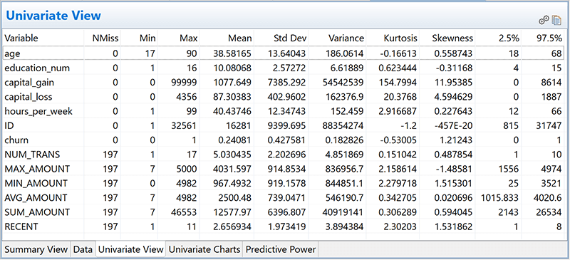
Figure 2. EDA (univariate view)
Figure 3. EDA (characteristic analysis)
Following exploratory data analysis (EDA), the data is treated to increase its quality. Data cleansing requires good business and data understanding so organizations and teams can correctly interpret the data. This is an iterative process designed to remove, replace, modify, and rectify irregularities. Two major issues with unclean data are missing values and outliers – both these things can dampen model accuracy, making it imperative that teams and organizations have a solid data cleansing process in place.
Before a decision is made on how to treat missing values, we need to understand the reason for missing data and understand the distribution of missing data so we can categorize it as:
- Missing completely at random (MCAR);
- Missing at random (MAR); or
- Missing not at random (MNAR)
Missing data treatment often assumes MCAR and MAR, but NMAR data is more difficult to deal with. The list below provides common treatments ordered by complexity.
| Missing Data Treatment | Description |
|---|---|
| Leave missing data | Small percentage of missing values could be tolerated Missing values have special meaning and would be treated as a separate category |
| Delete missing data | Listwise (complete) or Pairwise Pros: simple and fast Cons: reduce statistical power, problematic on small datasets |
| Single imputation | Mean, mode, median; add missing_flag for adjustment; Pros: simple, fast and uses the complete dataset Cons: reduced variability, ignores relationship between variables; not effective where that data contains a large amount of missing values (typically more than 5% of the data) |
| Model-based imputation | Regression Pros: simple Cons: reduced variance KNN imputation Pros: imputes categorical and numeric data Cons: performance issue on large datasets Maximum likelihood estimation Pros: unbiased, used the complete dataset Cons: complex Multiple imputation Pros: accurate, cutting-edge machine learning technique Cons: difficult to code without a special function |
Table 3. Missing data treatments
Outliers are another “beast” in our data, since they can violate the statistical assumptions that underpin models. Once identified, it’s important to understand why outliers are there before applying any treatment, because while in most cases they must be dealt with, they can occasionally be useful. For example, outliers could be a valuable source of information in fraud detection; in that case, it’d be a bad idea to replace them with a mean or median value.
Outliers should be analyzed using univariate and multivariate analysis. For detection, we can use visual methods like histograms, box plots, or scatter plots; we can also use statistical methods like mean and standard deviation, clustering, small decision tree leaf nodes, Mahalanobis distance, Cook’s D, and/or Grubbs’ test. But determining what is and isn’t an outlier isn’t as simple as identifying missing values. The decision should be based upon a specified criterion. For example: any value outside ±3 standard deviations, or ±1.5IQR, or 5th to 95th percentile range would be labeled as an outlier.
Outliers can be treated in a similar way as missing values, but other transformations can also be utilized, including binning, weights assignment, conversion to missing values, logarithm transformations, and/or Winsorization.
As discussed above, data cleansing may require teams to implement different statistical and machine learning techniques. Even though these transformations could create better scorecard models, teams must consider the practicality of implementing these, since complex data manipulations can be costly, difficult to implement, and they can slow down model processing performance.
Once the data is clean, we’re ready for a more creative part – data transformation. Data transformation (or feature engineering) is the creation of additional (hypothesized) model variables that are tested for significance. The most common transformations include binning and optimal binning, standardization, scaling, one hot encoding, interaction terms, mathematical transformations (from non-linear into linear relationships and from skewed data into normally distributed data) and data reduction using clustering and factor analysis.
Apart from some general recommendations on how to tackle this task, it’s the data scientist’s responsibility to suggest the best approach to transform the customer data signature into the powerful mining view. This is probably the most creative – and most challenging – aspect of the data scientist’s role since it requires both a solid grasp of business understanding and considerable statistical and analytical ability. Often, the key of a good model isn’t the power of a specific modeling technique, but the breadth and depth of derived variables that represent a higher level of knowledge about the phenomena being examined.
Conclusion
Credit scoring is a dynamic, flexible, and powerful tool for lenders, but there are plenty of ins and outs that are worth covering in detail. To learn more about credit scoring and credit risk mitigation techniques, read the next installment of our credit scoring series, Part Four: Variable Selection.
Read prior Credit Scoring Series installments: